In the last post I showed how I imported a Whatsapp-conversation and tidied it up a bit. Now I want to analyze it. For that I will use the libraries dplyr, stringr and ggplot2.
As a first step, I format the dates properly and create some new columns. I also decide to just focus on two years, 2016 and 2017.
data=data%>%mutate(
  #convert DAte to the date format.
        Date=as.Date(Date, "%d.%m.%y"),
        year = format(Date,format="%y"),
        hour =  as.integer(substring(Time,1,2))
        #I filtered for two year, 2016/17
        )%>%filter(year=='17'|year=='16')
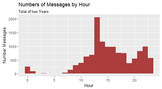
ggplot(data,aes(x=hour))+
  geom_histogram(fill="brown",binwidth=1,alpha=0.9)+
  labs(title="Numbers of Messages by Hour", subtitle="Total of two Years",
       y="Number Messages", x="Hour")
See more about the writing behavior of me an my friend, there is more formatting necessary. The words need to be counted too. To do so I use the stringr-library with str_count(data$Message, "\\S+")
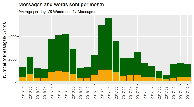
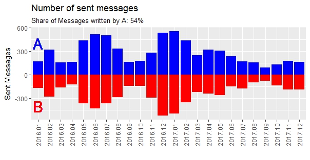
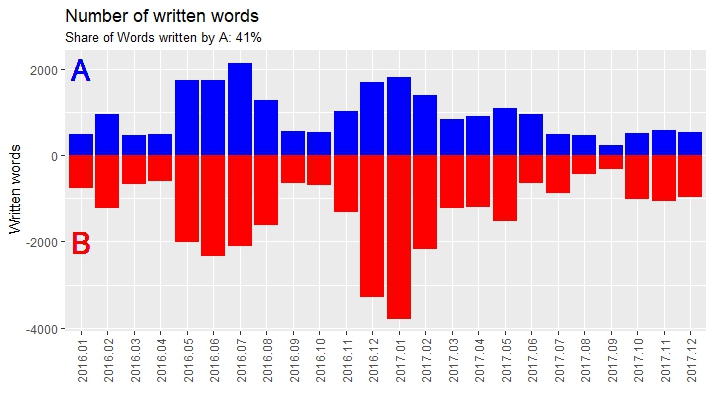
The rest of the reformatting is creating a binary variable for the author of the line, counting the words of each author and finally summarizing the data into groups containing one month of data.
wdata=data%>%mutate(
  #is later need for summarizing per month
        nmessage=1,
  #Counts number of words. (includes emojis as words) Space is the sperator
        nwords=str_count(data$Message, "\\S+"),
  #create binary variable for author
        AorB=ifelse(Author==nameA,1,0),
  #number of words/messages A
        Awords=AorB*nwords,
        Amessages=AorB*nmessage,
  #number of words/messages B
        Bwords=(AorB-1)*nwords,
        Bmessages=(AorB-1)*nmessage,
  #create month-variable with year
        month = format(Date,format="%Y.%m")
        )%>%
  #summarise by month
        group_by(month)%>%
        summarise(
          nwords = sum(nwords),
          nmessages=sum(nmessage),
          Awords=sum(Awords),
          Amessages=sum(Amessages),
          Bwords=sum(Bwords),
          Bmessages=sum(Bmessages),
          AorB=sum(AorB)
          )
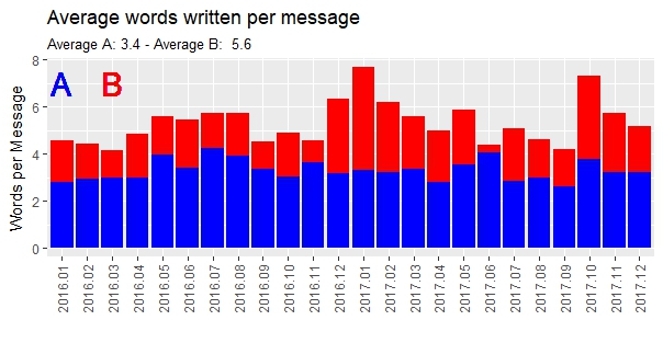
With this new data-frame, I can now easily create following graphs and look at the behavior of the people writing. There result are some interesting graphs. I am person A. I have the habit to write a lot of short messages. Which is clearly visible here. It probably should have been cleaned up more. Pictures, Videos and Gifs are still counted as words and so are emojis. I didn’t bother though, because the overall trends are still clearly visible.
Finally I wanted to know which words were used the most. I separated all the words and created a vector. I looked at the frequency with table().
words <- str_match_all( data$Message, "\\S+" )
#unlist the everything an make it lowercase
words=unlist(words)%>%tolower()
#make a table of the wordlist for freqency and make it a dataframe
wordfreq=data.frame(table(words))
#sort dataframe
wordfreq=wordfreq[order(wordfreq$Freq,decreasing=TRUE),]
The result isn’t too interesting. The conversation was conducted in Swiss-German, so there doesn’t exist any helpful word filters to get rid of all the particles and connection-words. That would be useful to make the result more meaningful.
words Frequency 1. i 1382 2. und 1037 3. de 789 4. so 538 5. ned 529
Here are the two most used emojis. (I didn’t figure out how to display them in R 🙁 )
-
smiling face with smiling eyes 🙂
-
grinning face with smiling eyes 😀
You can see the whole code here.